flowchart TD
    A[Bridge] -->|Height| B[Over 700 m]
    A -->|Height| C[Under 700 m]
    B -->|Location| D[Urban]
    B -->|Location| E[Non-urban]
    C -->|Location| F[Urban]
    C -->|Location| G[Non-urban]
    D -->|Traffic| H[X< per day]
    D -->|Traffic| L[<=X per day]
    E -->|Traffic| I[X< per day]
    E -->|Traffic| M[<=X per day]
    F -->|Traffic| J[X< per day]
    F -->|Traffic| N[<=X per day]
    G -->|Traffic| K[X< per day]
    G -->|Traffic| O[<=X per day]
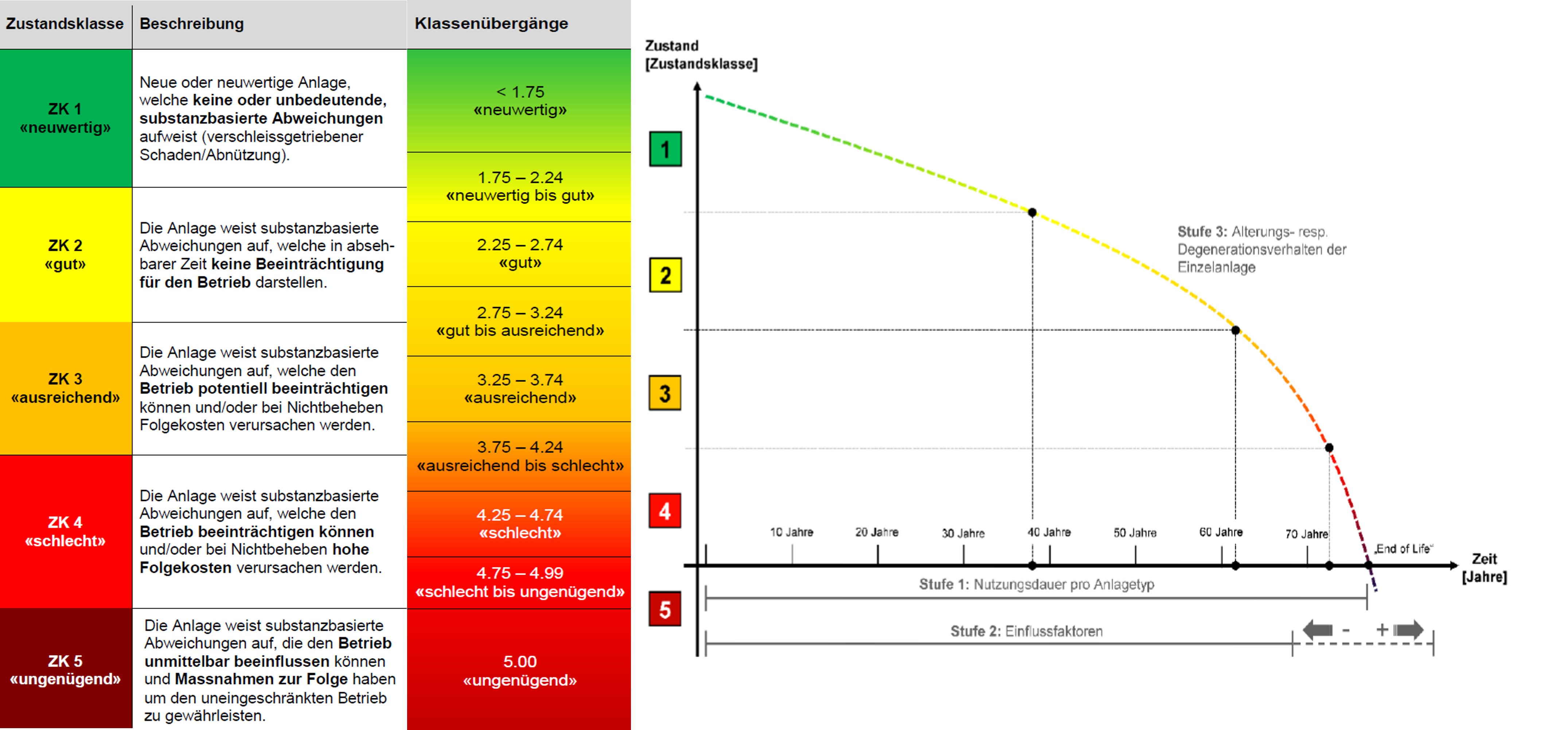
Define condition classes and model deterioration
Estimation of financial needs and condition of infrastructure assets
2024-03-11
Some questions
- How can we measure the deterioration?
- How fast do assets deteriorate?


Introduction – What has to be predicted?
Required
Provided
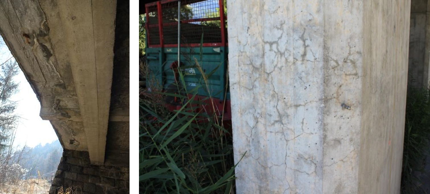
Gradual/Manifest
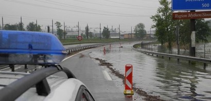
Sudden/Latent
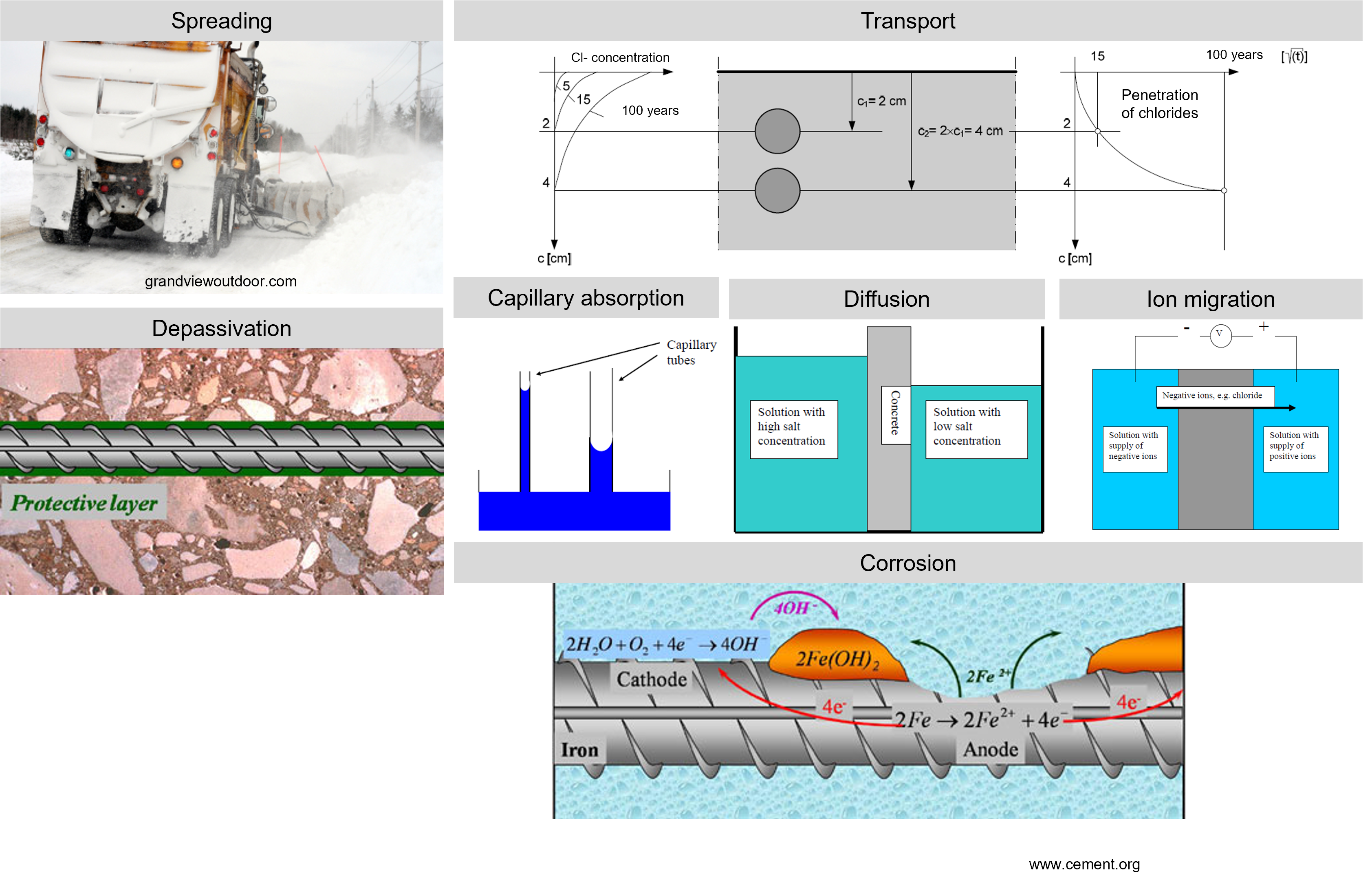
Introduction – Which processes do you want to consider? Chloride induced corrosion of steel
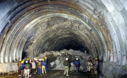
SZU example
How do we predict the future states of infrastructure if we consider the infrastructure to be in discrete states?
We can use a Markov model
Consider a sequence of random variables \({X_k, k = 0,1,2,….}\) , where each \(X_k\) can be one of a finite number of possible values, i.e. states.
These states are a set of non-negative integers from the set \(S = {1,2,…,n}\).
If \(X_k = i\), then the process (or Markov chain) is said to be in state \(i\) at time \(k\).

How do we predict the future states of infrastructure if we consider the infrastructure to be in discrete states?
We can use a Markov model
- The future condition state are predicted:
- State at \(\quad t+1=S(t)\cdot P\)
- State at \(\quad t+2=S(t+1)\cdot P\) \[ \vdots \]
- State at \(\quad t+n=S(t+(n-1))\cdot P\)

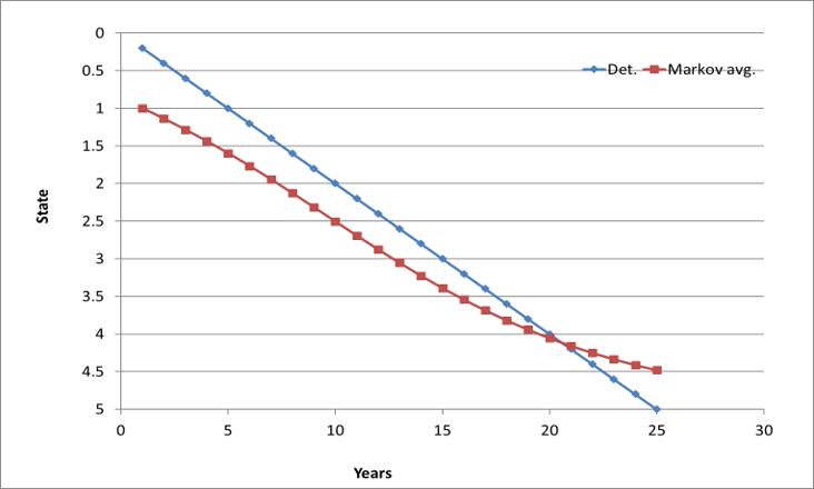
CS evolution between \(t = 0\) and \(t = 50\)
How do we estimate transition probabilities if we have data (at uniform inspection intervals)?
- In year \(t\) – number of items in \(S_i = X_i\)
- In year \(t+1\) - number of items moved from \(S_i\) to \(S_j\) \(= Y_{ij}\)
- Transition probability of remaining in \(S_i =\) \(Y_{ii}\over X_{i}\)
- Transition probability of moving from \(S_i\) to \(S_j=\) \(Y_{ij}\over X_{i}\) \(\forall i\neq j\).

How do we estimate transition probabilities if we have deterministic models and ensure a best fit?
| CS at \(t=0\)/\(t=t+1\) | 1 | 2 | 3 | 4 | 5 |
|---|---|---|---|---|---|
| 0 | 0.86 | 0.13 | 0 | 0 | 0 |
| 1 | 0 | 0.81 | 0.18 | 0 | 0 |
| 2 | 0 | 0 | 0.74 | 0.25 | 0 |
| 3 | 0 | 0 | 0 | 0.65 | 0.37 |
| 4 | 0 | 0 | 0 | 0 | 1 |
Next steps
- Today:
- Definition of the condition states
- Modelling the gradual deterioration
- Next step:
- Define possible interventions and strategies

Thank you for your attention!
Questions?
Hamed Mehranfar
Doctoral student
hmehranfar@ethz.ch
ETH Zürich
Institute of Construction and Infrastructure Management (IBI)
Chair of Infrastructure Management
HIL G 32.2, Stefano-Franscini-Platz 5
8093 Zürich

